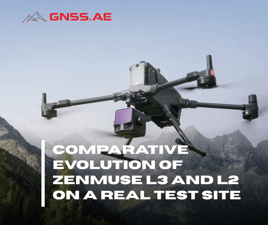
At GNSS.AE, practical validation is a key part of how we evaluate new technologies. To understand the real-world capabilities of the DJI Zenmuse L3, our engineering team conducted a controlled field test, directly comparing it with its predecessor, the Zenmuse L2.
This case study presents the results of that evaluation, focusing on measurable differences in point cloud density, noise levels, level of detail, and overall operational performance.
The field tests and data analysis were conducted by a GNSS.AE engineer, Bakhberde Adebiyet, in collaboration with the AERONEX team. During flights at 115 meters AGL, the Zenmuse L3 showed up to 96% lower noise levels compared to the L2.
These results raise a practical question: what enables such a difference in performance? To better understand this, we begin with a side-by-side comparison of the two sensors’ specifications, followed by an analysis of their behavior in real survey conditions.
System Specifications: DJI Zenmuse L3 vs. DJI Zenmuse L2
| Feature | DJI Zenmuse L3 | DJI Zenmuse L2 |
| Laser Wavelength | 1535 nm | 905 nm |
| Laser Beam Divergence | 0.25 mrad | Horizontal 0.2 mrad, Vertical 0.6 mrad |
| Laser Spot Size | Φ 41 mm@120 m (1/e²) Φ 86 mm@300 m (1/e²) | Horizontal 4 cm, vertical 12 cm @ 100 m (FWHM) |
| Detection Range | 950 m @ 10% reflectivity | 450 m @ 50% reflectivity |
| Laser Pulse Emission Frequency | up to 2000 KHz | 240 kHz |
| Returns per Pulse | Up to 16 (Multi‑return) | Up to 5 (Penta Return) |
| Camera System | Dual 100MP 4/3 CMOS | Single 20MP 4/3 CMOS |
| RGB Field of View | Linear: H – 80°, V – 3° Star-Shaped: H – 80°, V – 80° Non-Repetitive Scanning: H – 80°, V -80° | Repetitive: H – 70°, V – 3° Non-repetitive: H – 70°, V – 75° |
| Vertical Accuracy | Vertical Accuracy: 3 cm @ 120 m Horizontal Accuracy: 4 cm @ 120 m | Vertical: 4 cm @ 150 m Horizontal: 5 cm @ 150 m |

That’s what the specs say. Now let’s see what actually happens when you fly.
The test site was located in Fujairah, UAE — selected for its diverse terrain, representative of real-world surveying environments.
Why Fujairah?
The site integrates two key landscape types for LiDAR evaluation:
🏔 Mountainous terrain — steep slopes and elevation variation, ideal for evaluating vegetation penetration, point cloud consistency, and performance across complex topography performance in complex topography.
🏙 Urban area — includes mid-rise buildings, roads, and power lines. This allows evaluation of edge definition, noise on flat surfaces, and alignment accuracy in overlapping scans.

This combination provides a robust test environment for both the DJI Zenmuse L3 and L2,covering both natural and structured features.
Both sensors were flown under identical conditions to ensure a fair comparison.
Parameter | ||
Speed | 10 m/s | 10 m/s |
Laser Pulse Emission Frequency
| 350 KHZ | 200 KHZ |
Side overlap | 60% | 60% |
Forward overlap | 70% | 70% |
Altitudes | 85 m and 115 m | 115 m |
GSD | 0.45 and 1.15 cm/pix | 3.09 cm/pix |
Scan patterns | Non‑Repetitive, Linear, Star‑Shaped | Non‑Repetitive |
Returns | 5 | 5 |
RTK mode | On, (no GCPs) | On, (no GCPs) |
GNSS Base Station | D-RTK 3 Multifunctional Station | D-RTK 3 Multifunctional Station |
Drone Platform | DJI Matrice 400 | DJI Matrice 400 |
The only difference in hardware settings was the scan frequency:
Why GSD differs at the same altitude:
To ensure a fair sensor‑to‑sensor comparison, we used identical processing settings for both L2 and L3 datasets:
Processing steps:
Raw data → Trajectory Optimization → Point Cloud Generation
Importantly:

This approach ensures that the comparison reflects true sensor performance, without software enhancement.
We compared point cloud density in two ways:
For each sensor at each altitude, we selected multiple sample areas. Within each area, we evaluated three zones:
This approach captures spatial variability in point cloud density across the entire survey swath — from the center to the overlaps.

Across all test areas, the L3 delivered ~26% higher point density than the L2.
While the exact value varies depending on terrain and scan zone, the improvement remains consistent.
As expected, flying lower increases point density. The difference is consistent across all three measurement zones (nadir, half‑angle, overlap). At 85 m, density is approximately 34% higher than at 115 m.

At 115 m, density was significantly lower and more variable — in some areas by 70% or more compared to 85 m.

Why such a big difference in the mountains?
Two main reasons:
The L3 offers three scan patterns: Non‑Repetitive, Linear, and Star‑Shaped.

We tested all three at 115 m altitude to evaluate how each pattern affects point cloud density and uniformity.

For the Point Cloud Completeness assessment, a strip of trees and bushes within the survey area was selected as a reference feature for evaluating point cloud completeness.
The Linear pattern produced the most complete point cloud representation of vegetation. Due to its systematic and evenly spaced scan geometry, it distributes laser pulses uniformly across the entire swath (both along-track and cross-track). This results in more reliable capture of fine branches, gaps between leaves, and ground returns beneath vegetation, with fewer gaps and more consistent coverage across the canopy


The systematic nature of Linear scanning ensures that all parts of the surveyed area receive a similar sampling intensity. In contrast, the Non-Repetitive pattern may result in less uniform sampling of fine structural elements such as thin branches, especially in complex vegetation environments.


The Star-shaped pattern also performed well; however, it is more sensitive to platform motion. At higher flight speeds, minor gaps in coverage may appear due to the interaction between scan geometry and aircraft movement. For optimal results with the Star-shaped pattern, it is recommended to adjust flight speed accordingly.


Noise in a point cloud manifests as unwanted vertical or horizontal scatter – it makes flat surfaces appear rough, edges fuzzy, and complicates automatic classification. We evaluated noise in four real‑world scenarios:

1) 0° scan angle (nadir) — L3 achieves an astonishing 2 mm RMS noise, which is practically invisible. This means even subtle surface details (e.g., pavement cracks, thin cables) can be measured with confidence. L2 at 6.4 cm is still usable for many tasks, but small features may be lost in the scatter.


2) Half scan angle — Noise usually increases towards swath edges due to longer slant range and higher incidence angle. L3 keeps it under 1 cm (8 mm), while L2 is 7 cm.


3) Overlap between swaths — Here we measured noise level between two adjacent flight lines. L2 shows 8.9 cm, L3 reduces this to 1.4 cm.


4) Roof surface — Although the numerical improvement (32.5%) appears relatively small, the practical impact is clearly noticeable. The L3’s lower noise level (5.4 cm vs 8.0 cm for L2) leads to smoother roof surfaces, sharper structural edges, and fewer reconstruction artifacts. This directly improves quality and reduces post-processing effort.


In addition to quantitative metrics, we assessed the quality of infrastructure feature representation by comparing the point clouds for curb stones and speed bumps under identical flight parameters. The evaluation reflected both geometric fidelity and surface consistency, which are essential for engineering and road inspection applications.


Under the stated test conditions, both sensors delivered good results. Curbs and road transitions are clearly visible in both point clouds, with no major loss of detail.
However, differences become visible in surface quality:
For routine road inspections, both sensors are usable, but L3 reduces the need for manual cleaning and provides cleaner surfaces for automated extraction.
Surface roughness remained low for both sensors, with fine details like curb edges clearly defined even at 115 m AGL. However, the L3’s noise advantage becomes evident on low‑profile objects, where a small vertical feature can be obscured by point scatter.
We evaluated operational performance based on the mission parameters. The figures below are valid only for these specific settings – actual performance will vary with altitude, overlap, speed, and PRF.

Under identical flight parameters, the L3 demonstrated ~40% higher productivity
The combination of wider scan angle (800 vs 700) and higher pulse frequency allows (350KHz vs 240KHz) L3 to cover approximately 40% more area in the same altitude, flight speed and overlap settings. And this comes without sacrificing quality – in fact, GSD and density are both significantly better.
What if you match same GSD for both sensors?
If you adjust L3’s altitude to achieve the same GSD as L2 (~3 cm/pix), the L3 can fly much higher and/or faster – up to its maximum capability (350 kHz – 2,000 kHz PRF, up to 950 m range). In that scenario, the productivity gain grows to 2–5 times or more.
Overall, the results demonstrate that the DJI Zenmuse L3 provides reliable, high-density LiDAR data, suitable for a wide range of engineering, topographic, and infrastructure mapping applications where geometric accuracy and repeatability are critical.
Compared to its predecessor, the L2, the L3 shows significant improvements, particularly in point cloud density, noise levels, and completeness of the data, with performance gains exceeding 70%, while the GSD value of the L3 is three times higher. These results were obtained at the same fixed flight altitude for both sensors; when adjusted for required accuracy or GSD, the L3’s performance is expected to increase several-fold.
This field evaluation and data analysis were conducted by the GNSS.AE in collaboration with the AERONEX team.
Geospatial Engineer: Bakhberde Adebiyet (GNSS.AE)